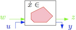
State-space models with 3 types of inputs and outputs

Systems in R-RoMulOC are defined in state-space. They can be continuous-time or discrete-time. The main difference with ss objects from the control toolbox is that three different types of inputs/outputs are defined.

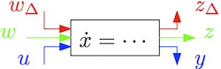
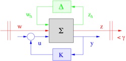
One pair of inputs/outputs is the classical control input (u) / measured output (y) pair. Default, when computing a feedback with some controller, these are the signals that are used to close the loop. The second pair of inputs/outputs (w/z) are intended for performance definition (guarantee for example an upper bound on the norm of the performance output z for norm bounded perturbations w). Finally, a pair (wd/zd) is used to define exogeneous feedback with uncertainties (used for LFT models). Notations for matrices of an ssmodel are as follows:

    dx =  A*x +  Bd*wd +  Bw*w +  Bu*u  
    zd = Cd*x + Ddd*wd + Ddw*w + Ddu*u  
     z = Cz*x + Dzd*wd + Dzw*w + Dzu*u  
     y = Cy*x + Dyd*wd + Dyw*w + Dyu*u  

Note that RoMulOC also allows the definition of arrays of systems, that is, a finite collection of models that share same dimensions of state, input and output vectors.

A typical and most simple way to declare a system in R-RoMulOC format is as follows:

>> sys = ssmodel('My plant');
>> sys.Bu = [1 0; 0 0.1 ; 0 0 ];
>> sys.A = [-1 0 0; 0.1 -2 0.2; 0.1 0.1 -1];
>> sys.Cy = [0 0 1];
>> sys.Bw = [1 ; 0 ; 0];
>> sys.Cz = [0 1 0];
>> sys
name: My plant
    	       n=3    mw=1    mu=2    
 n=3	dx  =   A*x +  Bw*w +  Bu*u
pz=1	 z  =  Cz*x                
py=1	 y  =  Cy*x                
continuous time ( dx : derivative operator )

>> sys.A

ans =

   -1.0000         0         0
    0.1000   -2.0000    0.2000
    0.1000    0.1000   -1.0000

Block diagonal uncertain operators

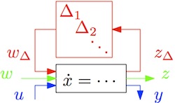
On of the two types of uncertain models considered R-RoMulOC is LFT modelling where the uncertainties enters the plant as a feedback loop. There can be multiple uncertainties all entering as a loop, thus defining a block diagonal uncertainty operator.

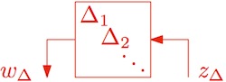
There are many types of uncertainties in R-RoMulOC providing many flexibilities. There is for example no need to a priori normalize these in set centered at zero and norm bounded by one. Moreover, the data you enter is kept the way you defined it, except if you decide to modify it. Below is an example involving two types of uncertainties. One is interval uncertainty which is a subcase of polytopes. The other is the classical norm-bounded uncertainty. Both can be combined in a block diagonal operator where blocks can be repeated and need not to be ordered.

>> di = uinter( [-1 1; 0 1] , [1 -1; 0 -1] )
 wd = #1 * zd
index	size	repeat.	RorC	dist.	nature	
#1	2x2	1	real	det.	LTI	interval 3 param	

>> dp = upoly( d1 )
 wd = #2 * zd
index	size	repeat.	RorC	dist.	nature	
#2	2x2	1	real	det.	LTI	polytope 8 vertices	

>> dn = unb( 1, 2, 1.2 )
 wd = #3 * zd
index	size	repeat.	RorC	dist.	nature	
#3	1x2	1	real	det.	LTI	norm-bounded by 1.2	

>> D =  diag( di, dn, di )
diagonal structured uncertainty
size: 5x6 | nb blocks: 3 | independent blocks: 2
 wd = diag( #1 #3 #1 ) * zd
index	size	repeat.	RorC	dist.	nature	
#1	2x2	2	real	det.	LTI	interval 3 param	
#3	1x2	1	real	det.	LTI	norm-bounded by 1.2	

LTI systems with uncertainties

There are two types of uncertain models in R-RoMulOC, namely LFT models and polytopic models. Both are contained in the ussmodel object. LFT models are defined as a feedback loop of some uncerttainty on the zd/wd exogeneous signals of the plant.

An example of LFT-type uncertain system definition is given below:

>> sys = ssmodel;
>> sys.A = -eye(3);
>> sys.Bd = eye(3);
>> sys.Cd = ones(3,3);
>> sys.Ddd = 0.1*ones(3,3);
>> d1 = unb(2,2,1.2);
>> d2 = uinter(-1,1);
>> D = diag(d1,d2);
>> usys = ussmodel( sys, D)

Uncertain model : LFT
-------- WITH --------
    	       n=3     md=3    
 n=3	dx  =   A*x +  Bd*wd
pd=3	zd  =  Cd*x + Ddd*wd
continuous time ( dx : derivative operator ) 
-------- AND  --------
diagonal structured uncertainty
size: 3x3 | nb blocks: 2 | independent blocks: 2
 wd = diag( #1 #2 ) * zd
index	size	repeat.	RorC	dist.	nature	
#1	2x2	1	real	det.	LTI	norm-bounded by 1.2	
#2	1x1	1	real	det.	LTI	interval 1 param	

The second type of uncertain systems is the class of polytopic systems, which include as special cases the parallelotopes and the intervals.

An example of such models is given below:

>> sys1 = ssmodel;
>> sys1.A = [-1 1;0 -1];
>> sys2 = ssmodel;
>> sys2.A = [1 -1;0 1];
>> usysi = uinter( sys1, sys2)

Uncertain model : interval 3 param
-------- WITH --------
    	       n=2    
 n=2	dx  =   A*x
continuous time ( dx : derivative operator ) 

>> usysp = upoly(usysi)

Uncertain model : polytope 8 vertices
-------- WITH --------
    	       n=2    
 n=2	dx  =   A*x
continuous time ( dx : derivative operator ) 

>> usysp(4).A

ans =

     1    -1
     0    -1

Analysis and control design problems

Once some plant (or several) plants have been defined in R-RoMulOC, building LMIs for some control problem to be solved is a matter of one line of code. In the example below we assume some uncertain plant has been defined (it is the one coded in the romuloc(1) demo). Four H-infinity computations are done. The first one gives the norm of the nominal plant. The second, based on randomized Monte-Carlo techniques gives a lower bound on the worst case. The third one is LMI-based with a unique Lyapunov matrix over all uncertainties, it gives an upper bound on the worst case. The last one is with parameter-dependent Lyapunov functions, it is less conservative and provides an improved upper bound.

>> usinf
Uncertain model : LFT
-------- WITH --------
name: shaped model
    	       n=8     md=6    mw=2    
 n=8	dx  =   A*x +  Bd*wd +  Bw*w
pd=7	zd  =  Cd*x + Ddd*wd + Ddw*w
pz=1	 z  =  Cz*x + Dzd*wd        
continuous time ( dx : derivative operator ) 
-------- AND  --------
diagonal structured uncertainty
size: 6x7 | nb blocks: 4 | independent blocks: 4
 wd = diag( #3 #4 #5 #6 ) * zd
index	size	repeat.	RorC	dist.	nature				name
#3	1x2	1	real	det.	LTI	{X,Y,Z}-dissipative	Inertia
#4	2x2	1	real	det.	LTI	norm-bounded by 0.25	Damping
#5	1x1	1	real	det.	LTI	interval 1 param	Input
#6	2x2	1	real	det.	LTI	polytope 3 vertices	Output

>> Hi_1 = norm( usinf, Inf )
Nominal 
Hi_1 =

    1.6027
	
>> pb2 = ctrpb('analysis','rand') + hinfty( usinf );
>> Hi_2 = solvesdp( pb2 )

459 tested random values out of 459 | worst case performance = 2.480e+00 

Hinfty norm = 2.48034 is the worst case estimate
The probability P for an other sample to violate the estimate is such that
  Prob{ P > 0.01 } less than 0.01

Hi_2 =

    2.4803	
	
>> pb3 = ctrpb('analysis') + hinfty( usinf )

control problem: ANALYSIS 
Lyapunov function: UNIQUE (quadratic stability)
Specified performances / systems:
# minimize HINFTY / shaped model

>> Hi_3 = solvesdp( pb3 )
[...computation...]

Hinfty norm less than 2.86659 assessed

Hi_3 =

    2.8666
	
pb4 = ctrpb('analysis','PDLF') + hinfty( usinf )

control problem: ANALYSIS 
Lyapunov function: QUADRATIC-LFT
Specified performances / systems:
# minimize HINFTY / shaped model

>> Hi_4 = solvesdp( pb4 )
[...computation...]

Hinfty norm less than 2.52258 assessed

Hi_4 =

    2.5226

Regions for robust pole location

In RoMulOC stability and pole location specifications are internally coded in a unified manner. Stability of continuous-time systems is the pole location in the left half of the complex plane. Stability of discrete-time systems is the pole location in the unit disc centered at the origin. Other pole location regions that may be defined are half planes that pass by any point of the complex plane and with any inclination with respect to the imaginary axis and discs centered at any point of the complex plane and with any radius. 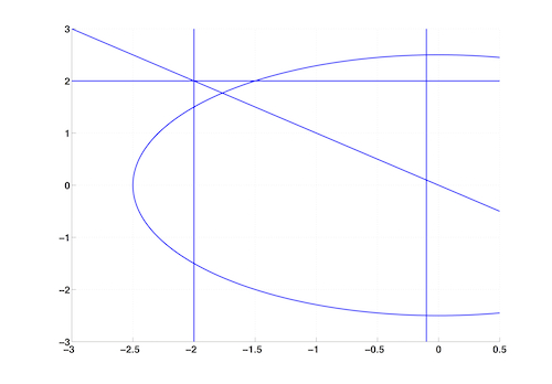Some examples or regions are as follows (with their interpretation on the modes of continuous time systems):
- a half plane such that the real part of the poles is less than -0.1 (guarantees time constant to be less than 10s).

>> r1 = region('plane',-0.1,0);

- a half plane such that the real part of the poles is greater than -2 (guarantees time constant to be greater than 0.5s).

>> r2 = region('plane',-2,pi);

- a half plane crossing the origin with angle of 45deg with respect to the imaginary axis (guarantees damping to be greater than sin(pi/4)=0.7071).

>> r3 = region('plane',0,pi/4);

- a half plane crossing 2j with angle of 90deg with respect to the imaginary axis (guarantees damped natural frequency to be less than 2rad/s).

>> r4 = region('plane',2j,pi/2);

- a disc centered the origin with radius 2.5 (guarantees natural frequency to be less than 2.5rad/s).

>> r5 = region('disc',0,2.5);

The regions can be plotted as follows.

>> axis([-3 0.5 -3 3]), grid, hold on
>> plot(r1), plot(r2), plot(r3), plot(r4), plot(r5)

Matrix ellipsoids - generaliation of norm-bounded constraints

Robustness is in the litterature most often with respect to uncertain operators defined as norm bounded, that is, in the case of linear applications (matrices), uncertainties centered at zero and with bounded L2-induced norm by usually 1. A generalization of such sets of matrices is the case of sets defined by a quadratic matrix inequality. Some examples follow.

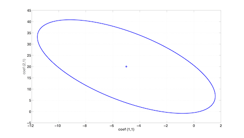
Ellipsoids of 2-by-1 matrices, that is of vectors of R^2.

>> e1=melli(-1,[1 -1],[1 0.2;0.2 0.1])
{X,Y,Z}-ellipsoid of real valued 2 x 1 matrices
>> center(e1)
ans =
   -5.0000
   20.0000
>> plot(e1);

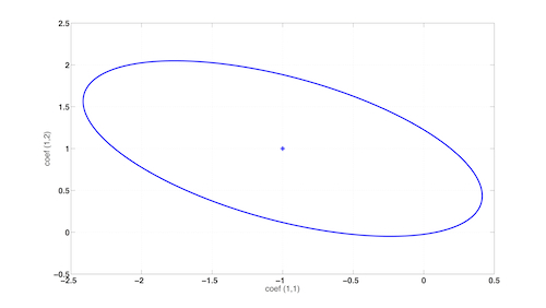
Ellipsoids of 1-by-2 matrices, which can by bijections be represented as vectors in R^2.

>> e2=melli([-1 -0.2;-0.2 -0.1],[1;-1],1)
{X,Y,Z}-ellipsoid of real valued 1 x 2 matrices
>> center(e2)
ans =
    -1     1
>> plot(e2);

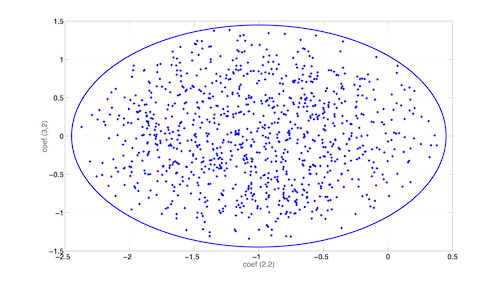
Ellipsoids of 3-by-2 matrices, for which one can plot projections on pairs of coefficients. It is also illustrated here that uniform sampling over such sets is made possible (uses sampling tools from RACT).

>> e3=melli([-1 -0.2;-0.2 -0.1],[1 0 1;-1 1 0],eye(3))
{X,Y,Z}-ellipsoid of real valued 3 x 2 matrices
>> center(e3)
ans =
    -1     1
     0    -1
    -1     0
>> plot(e3,2:3,2);
>> hold on
>> e3samples=usample(e3,1000);
>> plot(reshape(e3samples(2,2,:),1,[]),reshape(e3samples(3,2,:),1,[]),'+','LineWidth',3)