Reproducing the Benchmarks for our 2019 Paper

This post describes how to reproduce the experiments reported in our [Formats19] paper. We assume that you already installed Twina and a recent release of Tina. You can also install a Docker image containing all the necessary tools, scripts and model files:

docker pull vertics/twina

In our experiments, we want to compare the results obtained with Product TPN (using Twina) and an encoding into IPTPN. By default, Twina uses option -W, that computes the Linear SCG of a net. We also provide option -I to compute the LSCG for the product of two nets.

Twina accepts the same input format for nets than Tina. In particular, our method can be used with nets that are not 1-safe and without any restriction on the timing constraints (so we accept right-open transitions). We also allow read- and inhibitor-arcs with the same semantics than in Tina.

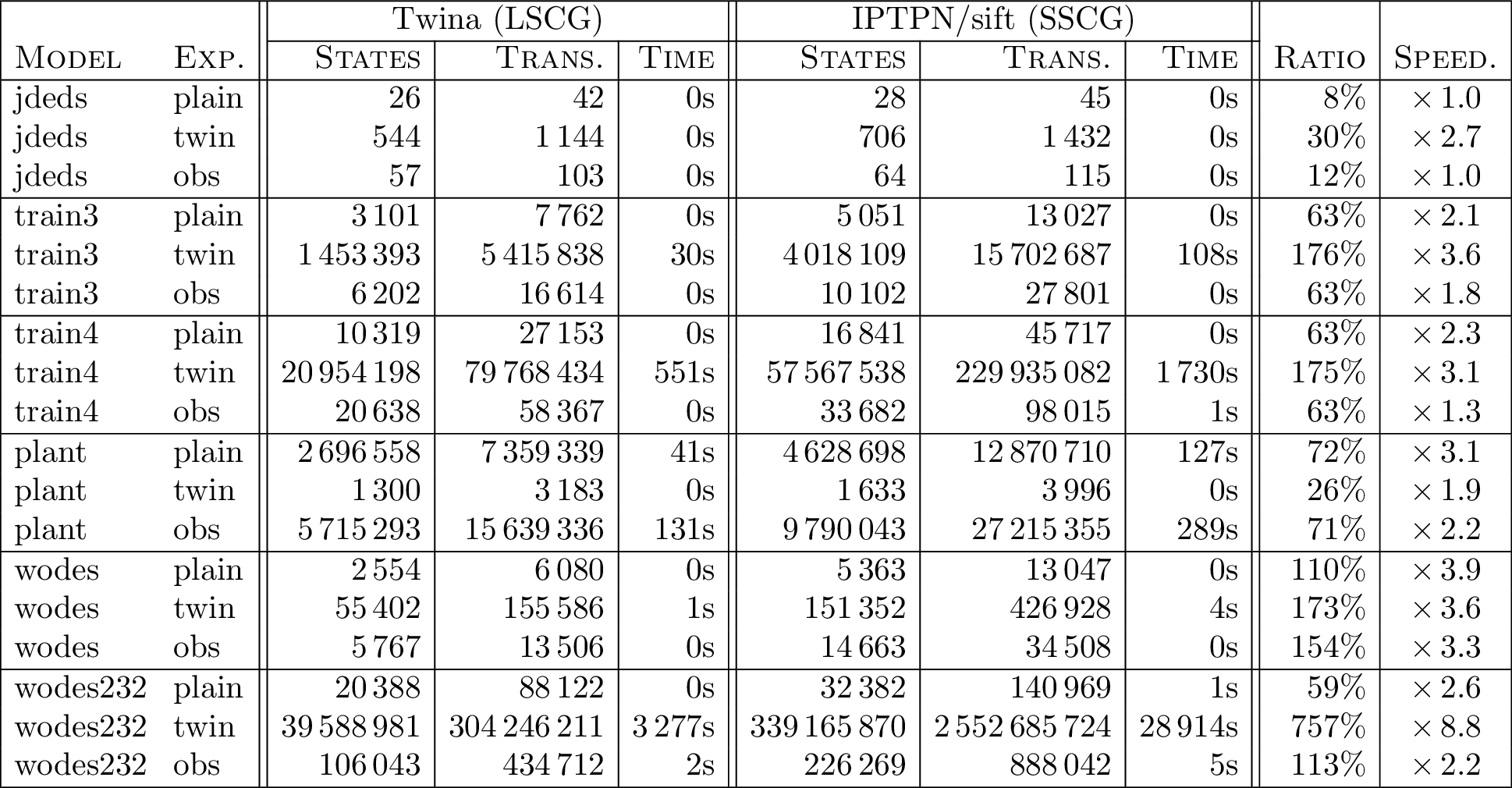
In the following, we compare the size of the LSCG obtained on different models with the results obtained using IPTPN and Tina. The results are reported in Fig. 1 below, with the sizes of the SCG in number of classes and edges; we also give the ratio of classes saved between the LSCG and the SSCG (so a ratio of 100% means that we have twice as much classes in the SSCG than in the LSCG). We use the sift tool to compute the SSCG from an IPTPN; sift is an optimized version of tina that provides fewer options (state class abstractions) but is much faster. Our table also reports the computation time for each test and the speedup. Computation time is not really relevant here though, since we compare two different tools.

We use different models for our benchmarks (in each case we state the name of the fault option used in the twin product construction):

• plant is the model of a complex automated manufacturing system from [Wang2015] (-fault=F);
• jdeds is an example taken from [DEDS17] extended with time (-fault=f);
• train is a modified version of the train controller example in the Tina distribution with an additional transition that corresponds to a fault in the gate (we have examples with 3 and 4 trains) (-fault=F1);
• wodes is the WODES diagnosis benchmark of Giua (found for instance in [DEDS17]) with added timing constraints (-fault=F1).

For each model, we give the result of three experiments: plain where we compute the SCG of the net, alone; twin where we compute the intersection between the TPN and a copy of itself with some transitions removed; and obs where we compute the intersection of the net with a copy of the observer that we discuss in another post on formal verification.

We provide a shell script to simplify the task of performing the benchmarks (see twinaluate.sh ). The whole environment is also distributed as a Docker file (all the models are included in the image), so you may only use a command like:

docker run vertics/twina ./twinaluate.sh train3 F1

Another shell script, benchmark.sh , can be used to generate a CSV file with all our results and correct headers. This file can be used to automatically generate the table that appear in our paper using LaTeX and the pgfplotstable package, see file table.tex)

$ ./benchmark.sh > data.csv
$ pdflatex -shell-escape table.tex

Examples used in this post

You can download all the files as a single ZIP archive benchmark.zip .