How to Use Twina

You can find a list of possible options for the tool using option -h.

$ twina -h
Usage of twina.exe:
  -I     compute LSCG for the intersection of twin-nets
  -P     use product-nets instead of twin-nets when used with options -I or -twin
  -S     compute the Strong State Class Graph (SSCG) for one net, preserves LTL
  -W     compute the Linear State Class Graph (LSCG) for one net, preserves LTL (DEFAULT)
  -aut   transition system output (.aut format)
  -diag  test diagnosability for one fault and returns a counter-example if not (see option --fault=label)
  -fault=string label used in the twin machine construction (default "_")
  -iptpn output a net with IPTPN arcs then quit (set -p)
  -kaut  transition system with state properties encoded (.aut format)
  -lt    prints labeled transition properties
  -net   prints the net being evaluated
  -parse just parses and check input
  -twin  compute LSCG for the twin machine (see option --fault=label)
  -v     textual output (full)

files:
   infiles: input file is stdin when using -
   outfile: output is always on stdout
   errorfile: error are always printed on stderr

By default twina uses option -W, that computes the (Linear) State Class Graph, or LSCG for short, for the system given as input. The LSCG is a deterministic automata that defines exactly the possible traces of a system (when the TPN is bounded); hence the reason why the LSCG preserves linear time properties (LTL).

Basic Usage and Display Options

By default, Twina gives you some statistics on the size of the generated graph, while option -v gives you a full textual output of the LSCG, complete with information on timing constraints (in the form of Difference Bound Matrices). With option -lt you may also display the labels associated with the transitions that are fired. (In this case silent actions have label i.)

It is possible to generate an automaton view of the LSCG in the AUT format (option -aut), the LTS description format of the Aldebaran tool of the CADP toolset. This format can be used with NetDraw. There is also option -kaut to export a specification in AUT format in which state properties (markings) are encoded as simple loops; see option -sp 2 of tina. This option is useful if you need to test the equivalence between different State Class Graphs or to export the result in the KTZ format, a compressed format for transition system used in the Tina toolbox.

Intersection (option -I)

Twina can generate a LSCG for the (synchronous) product of two TPN, that is a state class graph containing only the executions that are common to both nets. Intuitively, a trace is common to two nets A and B if we can find a pair of executions, $(\sigma_A, \sigma_B)$, one in each net, such that any labelled transition in $\sigma_A$ can be uniquely matched to a transition with the same label in $\sigma_B$, at the same date and in the same order (and vice versa).

When the two nets have the same set of labels (same alphabet) the set of common traces corresponds to language intersection. This methods can be used even when the two TPN have transitions sharing the same label and that have a non-trivial timing constraints (i.e. different from $[0, +\infty[$); that is even if we cannot compose the two nets together.

You can generate the LSCG for the intersection of two TPN using option -I. For example, if we consider the running example of [Formats19] (see files C1.net and C2.net ).

$ twina -v -lt -I  C1.net C2.net
# states 3
# transitions 2

class 0
  marking: {p0.1} {p1.1} {p0.2}
  domain:
   0 <= {t0.1} <  w
   0 <= {t1.1} <= 1
   0 <= {t0.2} <  w
  successors: {t0.1}|{t0.2}:"a"/1

class 1
  marking: {p1.1} {p1.2}
  domain:
   0 <= {t1.1} <= 1
   1 <= {t1.2} <  w
  successors: {t1.1}|{t1.2}:"b"/2

class 2
  marking:
  domain:
  successors:

In the resulting SCG, places and transitions from the first net are suffixed with .1, and are suffixed with .2 for the second net. We can see from the result that, initially, only transitions labelled with a can be fired (i.e. t0 from C1 at the same time than t0 from C2). This corresponds to the “product” transition {t0.1}|{t0.2} in the product TPN. Looking at the timing constraints, we can also deduce that these transitions should fire before 1 unit of time.

Twin-Plant Method for TPN (options -twin and -diag)

It is possible to distinguish a particular label, say f, using option --fault=f. This fault label can be interpreted as the label of actions corresponding to a silent failure in the system.

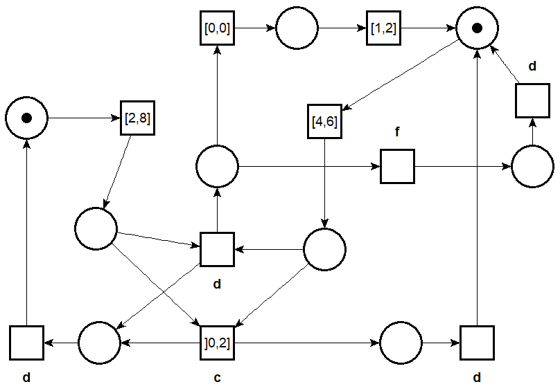
The twin-plant of a net, A, is defined as the product of A with a copy of itself where every transitions labelled with the fault f have been removed. For instance, this is the result of analyzing the twin-plant for model jdedstimed that is part of our examples.

$ twina -twin -fault=f jdedstimed.net
544 classe(s), 121 marking(s), 489 domain(s), 1144 transition(s)
0.004s

This construction is interesting since the twin plant can be used to check if there are failed executions in A (meaning executions that have triggered a fault) that can be mistaken with non-faulty one. In this case one can say that the net is not diagnosable.

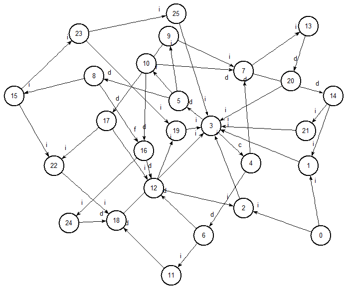
It is possible to detect that a system is not diagnosable without generating all the reachable classes of a net. Indeed, it is enough to stop when we find an inifinite trace (a loop) that contains label f in the LSCG of the twin machine. To this end, we have implemented a dedicated on-the-fly diagnosability check in Twina (see option -diag).

In our example, we find that the system is not diagnosable after generating only 110 classes. It is also possible to print (a textual representation of) the counter-example using option -v.

$ twina -diag --fault=f  jdedstimed.net

# net is not diagnosable
# length:              40
#
# states (explored):   110
# markings:            57
# dbms:                97
0.000s

$ twina -diag --fault=f -v -lt jdedstimed.net
# net is not diagnosable
# length: 40
class 0
  marking: {p0.1} {p1.1} {p0.2} {p1.2}
  domain:
   2 <= {t0.1} <= 8
   4 <= {t1.1} <= 6
   2 <= {t0.2} <= 8
   4 <= {t1.2} <= 6
----[{t0.1}:"i"]--------->
class 1
  marking: {p2.1} {p1.1} {p0.2} {p1.2}
  domain:
   0 <= {t1.1} <= 4
   0 <= {t0.2} <= 6
   0 <= {t1.2} <= 4
   {t1.1} - {t1.2} <= 2
   {t0.2} - {t1.1} <= 4
   {t0.2} - {t1.2} <= 4
   {t1.2} - {t1.1} <= 2
----[{t1.1}:"i"]--------->

[...]

We still have some limitations at the moment. For instance, Twina may return a “non-optimal” counter-example (not among the shortest ones). We may also return a counter-example where the fault needs to be fired an unbounded number of times. We plan to provide new options in order to overcome these limitations.

Inhibition-Permission TPN (options -iptpn)

There is already an extension of TPN, available in Tina, that can be used to “compute the product of two nets” even when they are not syntactically composable. In this extension, called IPTPN, we can use two new kinds of arcs between transitions: one that can inhibit a transition (akin to a priority); and the dual relation, where a transition can “permit” another one to fire. This extension has been detailed in [DEDS2011].

Unlike our approach, IPTPN are strictly more expressive than TPN and they require to use a more precise State Class Graph construction called SSCG (for Strong SCG). It is possible to check nets with IPTPN arcs in Tina by declaring a shell variable called IPTPN in your environment.

To compare the two aproaches, we provide the possibility to generate an IPTPN net from a twin-plant or the intersections of two TPN. This net (in tpn format) can be directly passed to Tina on the standard input. This option supports input nets that have priorities between transitions.

$ export IPTPN=1
$ twina --fault=f -twin -iptpn jdedstimed.net | sift -
121 marking(s), 398 domain(s), 706 classe(s), 1432 transition(s)
0.016s

In this case, the strong SCG (SSCG) has 706 classes, compared to only 544 classes in the LSCG computed by Twina. Indeed, it is often the case that the strong SCG has far more classes than the related linear one.